
Understanding Contrast Algorithms
As a hobbyist photographer, I’ve always wondered how Apple Photos, Lightroom, and Photoshop implement image contrast adjustments. After spending some time reading into it, the approach is worth sharing.
Let’s start with the basics.
A histogram is simply a bar chart representing [in this case] different frequencies of colors in an image.
Here’s a typical histogram you might see:
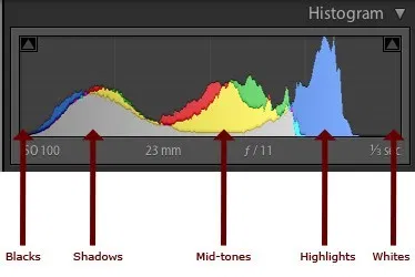
Source: Histograms for Beginners
Brightness
As a preliminary step, let’s try and manipulate the brightness in an image. It’ll lend itself to making contrast adjustments later on.
Given a histogram, if we shift it’s contents left or right, we can make the image darker or lighter respectively.
Let’s assume we’re dealing with 8-bit RGB color space. One side of the histogram would be (0, 0, 0) [black] and the other side would be (255, 255, 255) [white].
As we move the histogram to the right, we increase the frequency of values closer to white in the image thereby brightening the image. Conversely, shifting the histogram to the left moves more of the values towards black, thereby darkening the image.
Here’s an example of a function that can shift the brightness of an image.
Original Image
Brightness + 40%
Brightness – 40%

The previous code is overly simplistic. A proper implementation would map the RGB color space to HSL. Then, it would modify the luminance values and then convert the image back to the RGB color space. However, modifying the RGB values in this way still illustrates the point without increasing the article’s scope.
Contrast
Contrast is really just a measure of the difference between the maximum and minimum pixel intensities in an image. So, in order to increase the contrast in an image, we need to increase the distance between the maximum and minimum pixel intensities.
We’ll take a look at a few different contrast adjustment algorithms starting with contrast/histogram stretching.
Contrast Stretching / Histogram Stretching
As the name implies, this is really just the process of taking the existing intensity values in the image and “stretching” them to fit the entire range of potential values – [0, 255].
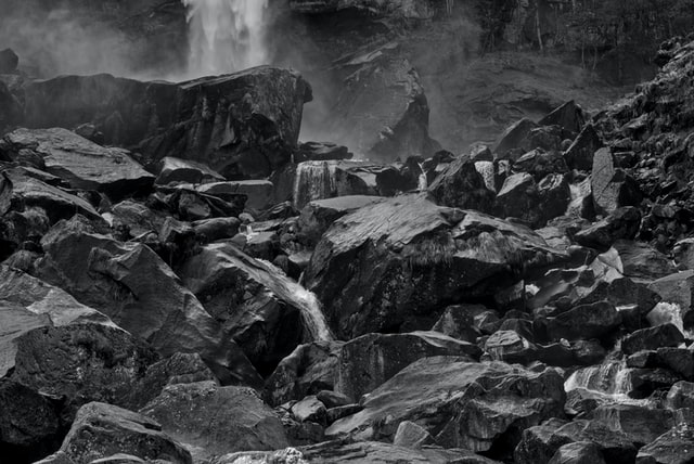
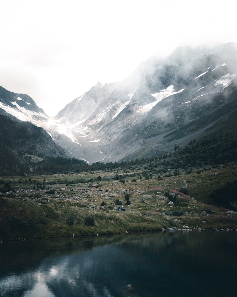
Photo by Giancarlo Corti on Unsplash
If we look at the image’s histogram, we’ll see that most of the intensity values are skewed to the left side of the graph and very few values exist in the higher intensity range.

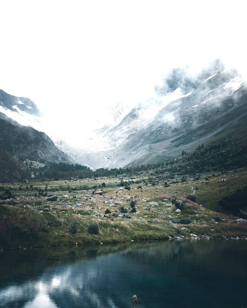
After applying contrast stretching to this photo, the histogram’s intensity values should be spread over this full range.
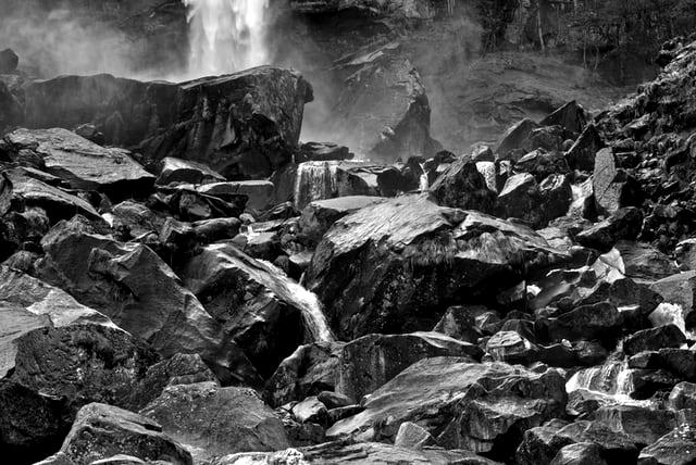
Since we’ve increased the difference between the maximum and minimum intensity values, you can see that we’ve increased the contrast in the image.
It’s also important to note that the general shape of the histogram is preserved with this approach. This won’t be the case with future algorithms we’ll look at.
To implement contrast stretching, we first need to find the minimum and maximum pixel intensities. Then, we can simply apply the following transformation on every pixel to get the new intensity value for that pixel in the output image.
If we wanted to apply this same approach to an RGB image, we’d need to convert the image to a Hue, Saturation, Intensity (HSI) color space. Then, we’d perform the same calculation above on just the Intensity value and then map the result back to the RGB color space.
The result of this normalization step would be a value between 0 and 1.0 which we’d then multiply by 255 to get the correct value for the pixel.
Code
There is one catch with this approach though.
Considering the formula above, we can see that if the min and max values were 0 and 255, the image is unaffected. So, most implementations of this algorithm pick values 5% from the edges instead of strictly the minimum / maximum intensity values.
You can always play with how far you move in from the edges to control how much additional contrast is applied to the image.

Source 
Histogram Stretching
Histogram Equalization
While histogram stretching modifies the range of intensity values to spread over the entire possible range, histogram equalization creates a uniform distribution of the histogram values.

Credit: Wikipedia
Histogram equalization by no means guarantees improved results. Converting the intensity values into a uniform distribution may very well decrease contrast or introduce additional noise into the image.
Pseudocode
- Iterate through all the pixels in the image
- Count the frequency of each intensity value in a dictionary.
- Create an empty array of length
256. - Using our dictionary, we’ll fill in this array such that each index stores the probability of that intensity value occurring in the source image. For example, index
5in the array will represent the probability with which an intensity of5appears in the input image. - Create a cumulative distribution function (we’ll go over this in a moment).
- Use the cumulative distribution function to transform the original pixel’s value and compute the new pixel value in the output image.
The first step is to count the various intensity frequencies in our source image:

The full code is available below, but here’s an excerpt of the output:
0, 3028
1, 1216
2, 1188
3, 1262
4, 1242
...
It shouldn’t be a surprise that the histogram values are heavily skewed to the left indicating the image is on the dark side.
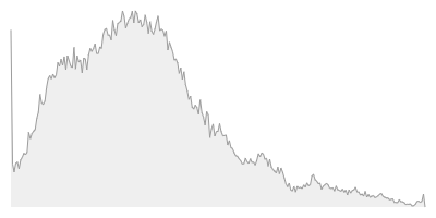
Now that we have our probability distribution, let’s generate our cumulative distribution function [CDF]. A CDF is a representation of how many values less than a certain value exist in our input image.
For example, in the chart below we can see that there’s approx. 150,000 pixels that are less than or equal to an intensity level of 65 (out of 255).
Calculating all of these frequencies and probabilities helps us in the transformation of the histogram into a uniform distribution.

Great! All we need to do is use the information in the CDF to transform the intensity values in the original image.
In order to perform this translation, we’ll take a pixel from the original image – for example, the pixel at (10, 10) – and we’ll find its intensity value. Then, we’ll use that intensity value to index into our array that is storing the results of the CDF to find the new intensity for the output pixel.
If this is still a little confusing, the code should clear things up.
Now, we have our new output image:

Let’s verify our work and look at the histogram of this new image:

Looks pretty uniform to me 🙂
Code
Alternatives
Let’s quickly cover some other approaches.
Nonlinear Stretching
When we were discussing contrast stretching, we were stretching all parts of the histogram equally. Nonlinear stretching is essentially the same approach, but it’ll use some other function to selectively stretch different parts of the histogram differently. For example, an implementation might use a logarithmic function to stretch the histogram instead.
Histogram Specification
This approach is closely related to histogram equalization. Instead of creating a uniform distribution, histogram specification enables you to transform an image’s histogram to match some other histogram you specify. So, histogram equalization is just one flavor of this approach where the provided histogram is uniformly distributed. Instead, this approach enables you to pass in any histogram to match.
Adaptive Histogram Modification
This approach involves creating several histograms that each correspond to different parts of the source image. This allows you to have much more granular contrast adjustments. This approach is often used when you want to provide local contrast adjustments or more generally refine the edges in your image.